eScience Lectures Notes : Line-Drawing Algorithms

Slide 1 : Line-Drawing Algorithms

Line-Drawing Algorithms

Introduction

Applications of Low-level Optimizations

More Low-level Optimizations (2)

More Low-level Optimizations (3)

Bresenham's line drawing algorithm

lineBresenham( ) Demonstration

Line-Drawing Algorithms

Our first adventure into scan conversion.
Scan-conversion or rasterization
Due to the scanning nature of raster displays
Algorithms are fundamental to both 2-D and 3-D computer graphics
Transforming the continuous into this discrete (sampling)
Line drawing was easy for vector displays

Line drawing is our first adventure into the area of scan conversion. The need for scan conversion, or rasterization, techniques is a direct result of scanning nature of raster displays (thus the names).
Vector displays are particularly well suited for the display of lines. All that is needed on a vector display to generate a line is to supply the appropriate control voltages to the x and y deflection circuitry, and the electron beam would traverse the line illuminating the desired segment. The only inaccuracies in the lines drawn a vector display resulted from various non-linearities, such as quantization and amplifier saturation, and the various noise sources in the display circuitry.
When raster displays came along the process of drawing lines became more difficult. Luckily, raster display pioneers could benefit from previous work done in the area of digital plotter algorithms. A pen-plotter is a hardcopy device used primarily to display engineering line drawings. Digital plotters, like raster displays, are discretely addressable devices, where position of the pen on a plotter is controlled by special motors called stepper motors that are connected to mechanical linkages that translates the motor's rotation into a linear translation. Stepper motors can precisely turn a fraction of a rotation (for example 2 degrees) when the proper controlling voltages are applied. A typical flat-bed plotter uses two of these motors, one for the x-axis and a second for the y-axis, to control the position of a pen over a sheet of paper. A solenoid is used to raise and lower the actual pen when drawing and positioning.
The bottom line is that most of the popular line-drawing algorithms used to on computer screens (and laser and ink-jet printers for that matter) were originally developed for use on pen-plotters. Furthermore, most of this work is attributed by a single man, Jack Bresenham, who was an IBM employee. He is currently a professor at Winthrop University.
In this lecture we will gradually evolve from the basics of algebra to the famous Bresenham line-drawing algorithms (along the same lines as a famous paper by Bob Sproull), and then we will discuss some developments that have happened since then.

Slide 3 : Vector Displays

Vector Displays

Oscilloscopes were some of the 1st computer displays
Used by both analog and digital computers
Computation results used to drive the vertical and horizontal axis (X-Y)
Intensity could also be controlled (Z-axis)
Used mostly for line drawings
Called vector, calligraphic or affectionately stroker displays
Display list had to be constantly updated
(except for storage tubes)

Tektronix 4014

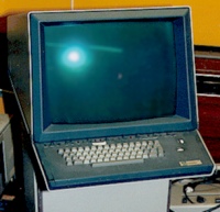
CRTs were embraced as output devices very early in the development of digital computers.

There close cousins, vacuum tubes, were some of the first switching elements used to build computers. Today, the CRT is a the last remaining vacuum tube in most systems (Even the flashing lights are solid-state LEDs). Most likely, oscilloscopes were some of the first computer graphics displays. The results of computations could be used to directly drive the vertical and horizontal displacement plates in order to draw lines on the CRT's face. By varying the current to the heating filament the output of the electron beam could also be controlled. This allowed the intensity of the lines to vary from bright to completely dark.
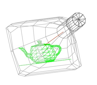
These early CRT displays were called vector, calligraphic or affectionately stroker displays. The demonstration above gives some feel for how they worked. By the way, this demo is an active Java applet. You can click and drag your mouse inside of the image to reorient the CRT for a better view. Notice the wireframe nature of the displayed image. This demo is complicated by the fact that it's a wireframe simulation of a wireframe display system. Notice how the color of the gray lines of the CRT vary from dark to light indicating which parts of the model that are closer to the viewer. This technique is called depth-cueing, and it was used frequently on vector displays.
The intensity variations seen on the teapot, however, are for a different reason. Eventually, the phosphors recover from their excited state and the displaced electrons return back to their original bands. The glow of the phosphor fades. Thus, the image on the CRT's face must be constantly redrawn, refreshed, or updated. The two primary problems with vector displays are that they required constant updates to avoid fading, thus limiting the drawn scene's complexity, and they only drew wireframes.

Slide 4 : pen-plotters

pen-plotters

Most incremental line-drawing algorithms were first developed for pen-plotters
Most of the early scan-conversion algorithms developed for plotters can be attributed to one man, Jack Bresenham.

Slide 5 : the Ideal Line

Quest for the Ideal Line

The best we can do is a discrete approximation of an ideal line.

Important line qualities:

Continuous appearence
Uniform thickness and brightness
Turn on the pixels nearest the ideal line
How fast is the line generated

Note that since vector-graphics displays, capable of drawing nearly perfect lines, predated raster-graphics displays. Thus, the expectations for line quality were set very high. The nature of raster-graphics display, however, only allows us to display a discrete approximation of a line, since we are restricted to only turn on discrete points, or pixels. In order to discuss, line drawing we must first consider the mathematically ideal line (or line segment).
From geometry we know that a line, or line segment, can be uniquely specified by two points. From algebra we also know that a line can be specified by a slope, usually given the name m and a y-axis intercept called b. Generally in computer graphics, a line will be specified by two endpoints. But the slope and y-intercept are often calculated as intermediate results for use by most line-drawing algorithms.
The goal of any line drawing algorithm is to construct the best possible approximation of an ideal line given the inherent limitations of a raster display.

Slide 6 : Simple Line

Simple Line

Based on the simple slope-intercept algorithm from algebra

y = m x + b

y0 = m x0 + b

y1 = m x1 + b

m = (y1 - y0)/(x1 - x0) = dy/dx

b = y0 - m x0

public void lineSimple(int x0, int y0, int x1, int y1, Color color) {
	int pix = color.getRGB();
	int dx = x1 - x0;
	int dy = y1 - y0;
	raster.setPixel(pix, x0, y0);
	if (dx != 0) {
		float m = (float) dy / (float) dx;
		float b = y0 - m*x0;
		dx = (x1 > x0) ? 1 : -1;
		while (x0 != x1) {
			x0 += dx;
			y0 = Math.round(m*x0 + b);
			raster.setPixel(pix, x0, y0);
		}
	}
}

The first line-drawing algorithm presented is called the simple slope-intercept algorithm. It is a straight forward implementation of the slope-intercept formula for a line.

Slide 7 : lineSimple( ) : Let's Make it Work!

Let's Make it Work!

Problem: lineSimple( ) does not give satisfactory results for slopes > 1

Solution: symmetry

public void lineImproved(int x0, int y0, int x1, int y1, Color color) {
	int pix = color.getRGB();
	int dx = x1 - x0;
	int dy = y1 - y0;
	raster.setPixel(pix, x0, y0);
	if (Math.abs(dx) > Math.abs(dy)) { // slope < 1
 		float m = (float) dy / (float) dx; // compute slope
		float b = y0 - m*x0;
 		dx = (dx < 0) ? -1 : 1;

		while (x0 != x1) {
 			x0 += dx;
			raster.setPixel(pix, x0, Math.round(m*x0 + b));
		}
	} else	if (dy != 0) { // slope >= 1
		float m = (float) dx / (float) dy; // compute slope
		float b = x0 - m*y0;
		dy = (dy < 0) ? -1 : 1;
		while (y0 != y1) {
			y0 += dy;
			raster.setPixel(pix, Math.round(m*y0 + b), y0);
		}
	}
}

It doesn't make sense to begin optimizing an algorithm before satisfies its design requirements! Code is usually developed under considerable time pressures. If you start optimizing before you have a working prototype you have no fall back position.
Our simple line drawing algorithm does not provide satisfactory results for line slopes greater than 1.

The solution: symmetry.

The assigning of one coordinate axis the name x and the other y was an arbitrary choice. Notice that line slopes of greater than one under one assignment result in slopes less than one when the names are reversed. We can modify the lineSimple( ) routine to exploit this symmetry as shown above.

Slide 8 : Optimize Inner Loops

Optimize Inner Loops

Optimize those code fragments where the algorithm spends most of its time.
Often these fragments are inside loops.
Overall code organization:

lineMethod( )	{
	// 1. general set up
	// 2. special case set up
	while (notdone)	{
		// 3. inner loop
	}
}

Remove unnecessary method invocations
replace
Math.round(m*x0 + b)
with
(int)(m*x0 + b + 0.5)
NB : does this always work?
Use incremental calculations
Consider the expression

y = (int)(m*x + b + 0.5)

The value of y is known at x0 (i.e. it is y0 + 0.5)
Future values of y can be expressed in terms of previous values with a difference equation:
yi+1 = yi + m;
or
yi+1 = yi - m;

The most important code fragments to consider when optimizing are those where the algorithm spends most of its time. Often these areas are within loops.
Our improved algorithm can be partitioned into two major sections. The first section is basically set-up code that is used by the second section, the central pixel-drawing while-loop. Most of the pixels are drawn in this while loop.

First optimization: remove unnecessary method invocations. Notice the call to the round class-method of the Math object that is executed for each pixel drawn. You might think that proper rounding is so trival a task that it hardly warrants a special method to begin with. But, it is complicated when differences between postive and negative numbers, and proper handling of fractions with a value of exactly 0.5 are considered.

However, in our line drawing code we are either not going to run into these cases (i.e. we only consider positive coordinate values) or we don't care (i.e. we don't expect to see values of 0.5 very often, and when we do we'd like to see them handled consistently). So for our purposes the call to Math.round(m*x0 + b) could be replaced with the following (int)(m*x0 + b + 0.5).

Second optimization: use incremental calculations.

Incremental or iterative function calculations use previous function values to compute future values. Often expressions within loops depend on a value that is being incremented or decremented on each loop iteration. In these cases the actual function values might be more efficiently calculated by first computing an initial value of the function during the loop set up, and updating the subsequent function values using a discrete version of a differential equation called a difference equation.

Consider the expression,
m*x0 + b + 0.5,
that is computed inside the first loop. The We can initialize the first value of the function outside of the loop:
y[0] = m*x0 + b + 0.5
. Future values of y depend only on how the value of x changes within the loop, since all other values are constant. Thus subsequent values of y can be computed by one of the following equations:
y[i+1] = y[i] + m; // if x0 is incremented

or
y[i+1] = y[i] - m; // if x0 is decremented
We can use a single equation if we change the sign of m, based on whether we are incrementing or decrementing, outside of the loop.

Last optimisation : use of integer operation instead of float one.

Slide 9 : Modified Algorithm

Modified Algorithm

This line drawing method is called a Digital Differential Analyzer or DDA for short.

public void lineDDA(int x0, int y0, int x1, int y1, Color color) {
	int pix = color.getRGB();
	int dy = y1 - y0;
	int dx = x1 - x0;
	float t = (float) 0.5; // offset for rounding
	raster.setPixel(pix, x0, y0);
	
	if (Math.abs(dx) > Math.abs(dy)) { // slope < 1
		float m = (float) dy / (float) dx; // compute slope
		t += y0;
		dx = (dx < 0) ? -1 : 1;
		m *= dx;
		while (x0 != x1) {
			x0 += dx; // step to next x value
			t += m; // add slope to y value
			raster.setPixel(pix, x0, (int) t);
		}
	} else { // slope >= 1
		float m = (float) dx / (float) dy; // compute slope
		t += x0;
		dy = (dy < 0) ? -1 : 1;
		m *= dy;
		while (y0 != y1) {
			y0 += dy; // step to next y value
			t += m; // add slope to x value
			raster.setPixel(pix, (int) t, y0);
		}
	}
}

Incorporating these changes into our previous lineImproved( ) algorithm gives the following result

Slide 10 : Low-Level Optimizations

Low-Level Optimizations

Low-level optimizations are dubious, because they depend on specific machine details.

However, a set of general rules that are more-or-less consistent across machines include:

Addition and Subtraction are generally faster than Multiplication.
Multiplication is generally faster than Division.
Using tables to evaluate discrete functions is faster than computing them
Integer caluculations are faster than floating-point calculations.
Avoid unnecessary computation by testing for various special cases.
The intrinsic tests available to most machines are greater than, less than, greater than or equal, and less than or equal to zero (not an arbitrary value).

Low-Level Optimizations
Low-level optimizations are somewhat dubious, because they depend on understanding various machine details. Because machines vary, the accuracy of these low-level assumptions can sometimes be questioned.
Typically, a set of general rules can be determined that are more-or-less consistent across machines. Here are some examples:
* Addition and Subtraction are generally faster than Multiplication.
* Multiplication is generally faster than Division.
* Using tables to evaluate discrete functions is faster than computing them
* Integer caluculations are faster than floating-point calculations.
* Avoid unnecessary computation by testing for various special cases.
* The intrinsic tests available to most machines are greater than, less than, greater than or equal, and less than or equal to zero (not an arbitrary value).
None of these rules are etched in stone. Some of these rules are becoming less and less valid as time passes. We'll address these issues in more detail later.

Slide 11 : Applications of Low-level Optimizations

Applications of Low-level Optimizations

For our line drawing algorithm we'll investigate applying several of these optimizations. The incremental calculation effectively removed multiplications in favor of additions. Our next optimization will use three of the mentioned methods. It will remove floating-point calculations in favor of integer operations, and it will remove the single divide operation (it makes a difference on short lines), and it will normalize the tests to tests for zero.

Notice that the slope is always rational (a ratio of two integers).

m = (y1 - y0) / (x1 - x0)

Note that the incremental part of the algorthim never generates a new y that is more than one unit away from the old one (because the slope is always less than one)

yi+1 = yi + m

Thus, if we maintained only the fractional part of y we could still draw a line by noting when this fraction exceeded one. If we initialize fraction with 0.5, then we will also handle the rounding correctly as in our DDA routine.

fraction += m; 
if (fraction >= 1) { 
	y = y + 1; fraction -= 1; 
}

Notice that the slope is always rational (a ratio of two integers).

m = (y1 - y0) / (x1 - x0)

Also note that the incremental part of the algorthim never generates a new y value that is more than one unit away from the old one, because the slope is always less than one (this assured by our improved algorithm).

y[i+1] = y[i] + m
Thus, if we maintained the only the only fractional part of y we could still draw a line by noting when this fraction exceeded one. If we initialize fraction with 0.5, then we will also handle the rounding correctly as in our DDA routine.

fraction += m
if (fraction >= 1) { y = y +1; fraction -= 1; }

Slide 12 : More Low-level Optimizations (2)

More Low-level Optimizations (2)

Note that y is now an integer.
Can we represent the fraction as an integer?
After we draw the first pixel (which happens outside our main loop) the correct fraction is:

fraction = 1/2 + dy/dx

If we scale the fraction by 2*dx the following expression results:

scaledFraction = dx + 2*dy

and the incremental update becomes:

scaledFraction += 2*dy         // 2*dx*(dy/dx)

and our test must be modified to reflect the new scaling

if (scaledFraction >= 2*dx) { ... }

Slide 13 : More Low-level Optimizations (3)

More Low-level Optimizations (3)

This test can be made a test against a value of zero if the inital value of scaledFraction has 2*dx subtracted from it. Giving outside the loop:

OffsetScaledFraction = dx + 2*dy - 2*dx = 2*dy - dx,

and the inner loop becomes

OffsetScaledFraction += 2*dy
if (OffsetScaledFraction >= 0) { 
	y = y +1; OffsetScaledFraction -= 2*dx; 
}

The net result is that we might as well double the values of dy and dx (this can be accomplished with either an add or a shift).

Slide 14 : Bresenham's line drawing algorithm

The resulting method is known as Bresenham's line drawing algorithm

public void lineBresenham(int x0, int y0, int x1, int y1, Color color) {
	int pix = color.getRGB();
	int dy = y1 - y0;
	int dx = x1 - x0;
	int stepx, stepy;
	if (dy < 0) { dy = -dy; stepy = -1; 
	} else { stepy = 1; 
	}
 	if (dx < 0) { dx = -dx; stepx = -1; 
	} else { stepx = 1; 
	}
	dy <<= 1; 							// dy is now 2*dy
	dx <<= 1; 							// dx is now 2*dx
 
	raster.setPixel(pix, x0, y0);

	if (dx > dy) {
		int fraction = dy - (dx >> 1);	// same as 2*dy - dx
		while (x0 != x1) {
			if (fraction >= 0) {
				y0 += stepy;
				fraction -= dx; 		// same as fraction -= 2*dx
			}
   		x0 += stepx;
   		fraction += dy; 				// same as fraction -= 2*dy
   		raster.setPixel(pix, x0, y0);
		}
	} else {
		int fraction = dx - (dy >> 1);
		while (y0 != y1) {
			if (fraction >= 0) {
				x0 += stepx;
				fraction -= dy;
			}
		y0 += stepy;
		fraction += dx;
		raster.setPixel(pix, x0, y0);
		}
	}
}

Slide 15 : Another look at Bresenham

Another look at Bresenham

from a more mathematical point of view...
...from computer code optimisation to geometry

main equations

(1) y = m x + b = DY/DX * x + b

y0 = m x0 + b

y1 = m x1 + b

(2) m = (y1 - y0)/(x1 - x0) = DY/DX

b = y0 - m x0

working hypothesis

(3) Let's consider for the demonstration that 0 <= m <= 1 and x0 < x1

<=> from one given step of the algo, we only have to chose between 2 pixels for the next step.

(and DX > 0)

which of two possible pixel positions is closer to the line path at each sample step

Slide 16 : Another look at Bresenham (2)

Another look at Bresenham (2)

decision : we'll study the sign of a integer parameter whose value is proportional to the difference between the separations of the two pixel positions from the actual line path.

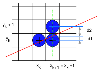
recursive process

step 0
from k to k+1 : choice (xk + 1, yk) or (xk + 1, yk + 1)

y = m (xk + 1) + b

d1 = y - yk = m (xk + 1) + b - yk

d2 = (yk + 1) - y = yk + 1 - m (xk + 1) -b

what we want to know : which of d1 and d2 is smaller, what we'll study : the sign of d1 - d2

d1 - d2 = 2 m (xk + 1) - 2 yk + 2b -1

Slide 17 : Another look at Bresenham (3)

Another look at Bresenham (3)

Let's get rid of float operations

the following decision parameter has the same sign as d1 - d2 :

(4) Pk = DX ( d1 - d2) = 2 DY . xk - 2 DX . yk + c = DX( 2 m (xk + 1) - 2 yk + 2b -1)
with c = constante = 2 DY + DX (2b -1)

Let's get rid of multiplications

Pk+1 = 2 DY . xk+1 - 2 DX .yk+1 + c

Pk+1 - Pk = 2 DY (xk+1 - xk) - 2 DX (yk+1 - yk) (get rid of the constance)

Pk+1 = Pk + 2 DY - 2 DX (yk+1 - yk)

Pk+1 = Pk + D'Y or = Pk + D'Y - D'X

with (yk+1 - yk) = 0 or 1 depending on Pk sign
(Pk < 0 <=> 0) and D'Y = 2 DY and D'X = 2 DX

P0 = 2DY - DX ( = 2 DY . x0 - 2 DX . y0 + 2 DY + DX (2b -1) )

(in our implemented algo, 'fraction' is the decision parameter Pk)

Slide 18 : Another look at Bresenham (4)

public void lineBresenham(int x0, int y0, int x1, int y1, Color color) {
	int pix = color.getRGB();
	int dy = y1 - y0;
	int dx = x1 - x0;
	int stepx, stepy;
	if (dy < 0) { dy = -dy; stepy = -1; 
	} else { stepy = 1; 
	}
 	if (dx < 0) { dx = -dx; stepx = -1; 
	} else { stepx = 1; 
	}
	dy <<= 1; 							// dy is now 2*dy
	dx <<= 1; 							// dx is now 2*dx
 
	raster.setPixel(pix, x0, y0);

	if (dx > dy) {
		int fraction = dy - (dx >> 1);	// same as 2*dy - dx
		while (x0 != x1) {
			if (fraction >= 0) {
				y0 += stepy;
				fraction -= dx; 		// same as fraction -= 2*dx
			}
   		x0 += stepx;
   		fraction += dy; 				// same as fraction -= 2*dy
   		raster.setPixel(pix, x0, y0);
		}			} else { ... }

Slide 19 : Life After Bresenham

Life After Bresenham

Possible configurations of the next two pixels
Most books would have you believe that the development of line drawing algorithms ended with Bresenham's famous algorithm. But there has been some signifcant work since then.

The following 2-step algorithm, developed by Xiaolin Wu, is a good example. The interesting story of this algorithm's development is discussed in an article that appears in Graphics Gems I by Brian Wyvill.

The two-step algorithm takes the interesting approach of treating line drawing as a automaton, or finite state machine. If one looks at the possible configurations that the next two pixels of a line, it is easy to see that only a finite set of possiblities exist.

The two-step algorithm also exploits the symmetry of line-drawing by simultaneously drawn from both ends towards the midpoint.

The code, which is further down this web page, is a bit long to show an a slide.

    public void lineTwoStep(int x0, int y0, int x1, int y1, Color color) {
        int pix = color.getRGB();
        int dy = y1 - y0;
        int dx = x1 - x0;
        int stepx, stepy;

        if (dy < 0) { dy = -dy;  stepy = -1; } else { stepy = 1; }
        if (dx < 0) { dx = -dx;  stepx = -1; } else { stepx = 1; }

        raster.setPixel(pix, x0, y0);
        raster.setPixel(pix, x1, y1);
        if (dx > dy) {
            int length = (dx - 1) >> 2;
            int extras = (dx - 1) & 3;
            int incr2 = (dy << 2) - (dx << 1);
            if (incr2 < 0) {
                int c = dy << 1;
                int incr1 = c << 1;
                int d =  incr1 - dx;
                for (int i = 0; i < length; i++) {
                    x0 += stepx;
                    x1 -= stepx;
                    if (d < 0) {                                               // Pattern:
                        raster.setPixel(pix, x0, y0);                          //
                        raster.setPixel(pix, x0 += stepx, y0);                 //  x o o
                        raster.setPixel(pix, x1, y1);                          //
                        raster.setPixel(pix, x1 -= stepx, y1);
                        d += incr1;
                    } else {
                        if (d < c) {                                           // Pattern:
                            raster.setPixel(pix, x0, y0);                      //      o
                            raster.setPixel(pix, x0 += stepx, y0 += stepy);    //  x o
                            raster.setPixel(pix, x1, y1);                      //
                            raster.setPixel(pix, x1 -= stepx, y1 -= stepy);
                        } else {
                            raster.setPixel(pix, x0, y0 += stepy);             // Pattern:
                            raster.setPixel(pix, x0 += stepx, y0);             //    o o 
                            raster.setPixel(pix, x1, y1 -= stepy);             //  x
                            raster.setPixel(pix, x1 -= stepx, y1);             //
                        }
                        d += incr2;
                    }
                }
                if (extras > 0) {
                    if (d < 0) {
                        raster.setPixel(pix, x0 += stepx, y0);
                        if (extras > 1) raster.setPixel(pix, x0 += stepx, y0);
                        if (extras > 2) raster.setPixel(pix, x1 -= stepx, y1);
                    } else
                    if (d < c) {
                        raster.setPixel(pix, x0 += stepx, y0);
                        if (extras > 1) raster.setPixel(pix, x0 += stepx, y0 += stepy);
                        if (extras > 2) raster.setPixel(pix, x1 -= stepx, y1);
                    } else {
                        raster.setPixel(pix, x0 += stepx, y0 += stepy);
                        if (extras > 1) raster.setPixel(pix, x0 += stepx, y0);
                        if (extras > 2) raster.setPixel(pix, x1 -= stepx, y1 -= stepy);
                    }
                }
            } else {
                int c = (dy - dx) << 1;
                int incr1 = c << 1;
                int d =  incr1 + dx;
                for (int i = 0; i < length; i++) {
                    x0 += stepx;
                    x1 -= stepx;
                    if (d > 0) {
                        raster.setPixel(pix, x0, y0 += stepy);                      // Pattern:
                        raster.setPixel(pix, x0 += stepx, y0 += stepy);             //      o
                        raster.setPixel(pix, x1, y1 -= stepy);                      //    o
                        raster.setPixel(pix, x1 -= stepx, y1 -= stepy);		        //  x
                        d += incr1;
                    } else {
                        if (d < c) {
                            raster.setPixel(pix, x0, y0);                           // Pattern:
                            raster.setPixel(pix, x0 += stepx, y0 += stepy);         //      o
                            raster.setPixel(pix, x1, y1);                           //  x o
                            raster.setPixel(pix, x1 -= stepx, y1 -= stepy);         //
                        } else {
                            raster.setPixel(pix, x0, y0 += stepy);                  // Pattern:
                            raster.setPixel(pix, x0 += stepx, y0);                  //    o o
                            raster.setPixel(pix, x1, y1 -= stepy);                  //  x
                            raster.setPixel(pix, x1 -= stepx, y1);                  //
                        }
                        d += incr2;
                    }
                }
                if (extras > 0) {
                    if (d > 0) {
                        raster.setPixel(pix, x0 += stepx, y0 += stepy);
                        if (extras > 1) raster.setPixel(pix, x0 += stepx, y0 += stepy);
                        if (extras > 2) raster.setPixel(pix, x1 -= stepx, y1 -= stepy);
                    } else
                    if (d < c) {
                        raster.setPixel(pix, x0 += stepx, y0);
                        if (extras > 1) raster.setPixel(pix, x0 += stepx, y0 += stepy);
                        if (extras > 2) raster.setPixel(pix, x1 -= stepx, y1);
                    } else {
                        raster.setPixel(pix, x0 += stepx, y0 += stepy);
                        if (extras > 1) raster.setPixel(pix, x0 += stepx, y0);
                        if (extras > 2) {
                            if (d > c)
                                raster.setPixel(pix, x1 -= stepx, y1 -= stepy);
                            else
                                raster.setPixel(pix, x1 -= stepx, y1);
                        }
                    }
                }
            }
        } else {
            int length = (dy - 1) >> 2;
            int extras = (dy - 1) & 3;
            int incr2 = (dx << 2) - (dy << 1);
            if (incr2 < 0) {
                int c = dx << 1;
                int incr1 = c << 1;
                int d =  incr1 - dy;
                for (int i = 0; i < length; i++) {
                    y0 += stepy;
                    y1 -= stepy;
                    if (d < 0) {
                        raster.setPixel(pix, x0, y0);
                        raster.setPixel(pix, x0, y0 += stepy);
                        raster.setPixel(pix, x1, y1);
                        raster.setPixel(pix, x1, y1 -= stepy);
                        d += incr1;
                    } else {
                        if (d < c) {
                            raster.setPixel(pix, x0, y0);
                            raster.setPixel(pix, x0 += stepx, y0 += stepy);
                            raster.setPixel(pix, x1, y1);
                            raster.setPixel(pix, x1 -= stepx, y1 -= stepy);
                        } else {
                            raster.setPixel(pix, x0 += stepx, y0);
                            raster.setPixel(pix, x0, y0 += stepy);
                            raster.setPixel(pix, x1 -= stepx, y1);
                            raster.setPixel(pix, x1, y1 -= stepy);
                        }
                        d += incr2;
                    }
                }
                if (extras > 0) {
                    if (d < 0) {
                        raster.setPixel(pix, x0, y0 += stepy);
                        if (extras > 1) raster.setPixel(pix, x0, y0 += stepy);
                        if (extras > 2) raster.setPixel(pix, x1, y1 -= stepy);
                    } else
                    if (d < c) {
                        raster.setPixel(pix, stepx, y0 += stepy);
                        if (extras > 1) raster.setPixel(pix, x0 += stepx, y0 += stepy);
                        if (extras > 2) raster.setPixel(pix, x1, y1 -= stepy);
                    } else {
                        raster.setPixel(pix, x0 += stepx, y0 += stepy);
                        if (extras > 1) raster.setPixel(pix, x0, y0 += stepy);
                        if (extras > 2) raster.setPixel(pix, x1 -= stepx, y1 -= stepy);
                    }
                }
            } else {
                int c = (dx - dy) << 1;
                int incr1 = c << 1;
                int d =  incr1 + dy;
                for (int i = 0; i < length; i++) {
                    y0 += stepy;
                    y1 -= stepy;
                    if (d > 0) {
                        raster.setPixel(pix, x0 += stepx, y0);
                        raster.setPixel(pix, x0 += stepx, y0 += stepy);
                        raster.setPixel(pix, x1 -= stepy, y1);
                        raster.setPixel(pix, x1 -= stepx, y1 -= stepy);
                        d += incr1;
                    } else {
                        if (d < c) {
                            raster.setPixel(pix, x0, y0);
                            raster.setPixel(pix, x0 += stepx, y0 += stepy);
                            raster.setPixel(pix, x1, y1);
                            raster.setPixel(pix, x1 -= stepx, y1 -= stepy);
                        } else {
                            raster.setPixel(pix, x0 += stepx, y0);
                            raster.setPixel(pix, x0, y0 += stepy);
                            raster.setPixel(pix, x1 -= stepx, y1);
                            raster.setPixel(pix, x1, y1 -= stepy);
                        }
                        d += incr2;
                    }
                }
                if (extras > 0) {
                    if (d > 0) {
                        raster.setPixel(pix, x0 += stepx, y0 += stepy);
                        if (extras > 1) raster.setPixel(pix, x0 += stepx, y0 += stepy);
                        if (extras > 2) raster.setPixel(pix, x1 -= stepx, y1 -= stepy);
                    } else
                    if (d < c) {
                        raster.setPixel(pix, x0, y0 += stepy);
                        if (extras > 1) raster.setPixel(pix, x0 += stepx, y0 += stepy);
                        if (extras > 2) raster.setPixel(pix, x1, y1 -= stepy);
                    } else {
                        raster.setPixel(pix, x0 += stepx, y0 += stepy);
                        if (extras > 1) raster.setPixel(pix, x0, y0 += stepy);
                        if (extras > 2) {
                            if (d > c)
                                raster.setPixel(pix, x1 -= stepx, y1 -= stepy);
                            else
                                raster.setPixel(pix, x1, y1 -= stepy);
                        }
                    }
                }
            }
        }
    }

Slide 20 : Epilogue

Epilogue

There are still many important issues associated with line drawing
Examples:

Non-integer endpoints (occurs frequently when rendering 3D lines)
Can we make lines appear less "jaggy" ?
What if a line endpoint lies outside the viewing area ?
How do you handle thick lines ?
Optimizations for connected line segments

eScience Lectures Notes : Line-Drawing Algorithms

Line-Drawing Algorithms

Let's Make it Work!

Line-Drawing Algorithms

Our first adventure into scan conversion.

Scan-conversion or rasterization

Due to the scanning nature of raster displays

Algorithms are fundamental to both 2-D and 3-D computer graphics

Transforming the continuous into this discrete (sampling)

Line drawing was easy for vector displays

Vector Displays

Oscilloscopes were some of the 1st computer displays

Used by both analog and digital computers

Computation results used to drive the vertical and horizontal axis (X-Y)

Intensity could also be controlled (Z-axis)

Used mostly for line drawings

Called vector, calligraphic or affectionately stroker displays

Display list had to be constantly updated (except for storage tubes)

Tektronix 4014

pen-plotters

Most incremental line-drawing algorithms were first developed for pen-plotters

Most of the early scan-conversion algorithms developed for plotters can be attributed to one man, Jack Bresenham.

Quest for the Ideal Line

The best we can do is a discrete approximation of an ideal line.

Important line qualities:

Continuous appearence

Uniform thickness and brightness

Turn on the pixels nearest the ideal line

How fast is the line generated

Simple Line

Based on the simple slope-intercept algorithm from algebra

y = m x + b

y0 = m x0 + b

y1 = m x1 + b

m = (y1 - y0)/(x1 - x0) = dy/dx

b = y0 - m x0

Let's Make it Work!

Problem: lineSimple( ) does not give satisfactory results for slopes > 1

Solution: symmetry

Optimize Inner Loops

Optimize those code fragments where the algorithm spends most of its time. Often these fragments are inside loops. Overall code organization:

Remove unnecessary method invocations replace Math.round(m*x0 + b) with (int)(m*x0 + b + 0.5) NB : does this always work?

Use incremental calculations Consider the expression y = (int)(m*x + b + 0.5) The value of y is known at x0 (i.e. it is y0 + 0.5) Future values of y can be expressed in terms of previous values with a difference equation: yi+1 = yi + m; or yi+1 = yi - m;

Modified Algorithm

This line drawing method is called a Digital Differential Analyzer or DDA for short.

Low-Level Optimizations

Low-level optimizations are dubious, because they depend on specific machine details.

However, a set of general rules that are more-or-less consistent across machines include:

Addition and Subtraction are generally faster than Multiplication.

Multiplication is generally faster than Division.

Using tables to evaluate discrete functions is faster than computing them

Integer caluculations are faster than floating-point calculations.

Avoid unnecessary computation by testing for various special cases.

The intrinsic tests available to most machines are greater than, less than, greater than or equal, and less than or equal to zero (not an arbitrary value).

Applications of Low-level Optimizations

Notice that the slope is always rational (a ratio of two integers).

Note that the incremental part of the algorthim never generates a new y that is more than one unit away from the old one (because the slope is always less than one)

Thus, if we maintained only the fractional part of y we could still draw a line by noting when this fraction exceeded one. If we initialize fraction with 0.5, then we will also handle the rounding correctly as in our DDA routine.

More Low-level Optimizations (2)

Note that y is now an integer. Can we represent the fraction as an integer? After we draw the first pixel (which happens outside our main loop) the correct fraction is:

If we scale the fraction by 2*dx the following expression results:

and the incremental update becomes:

and our test must be modified to reflect the new scaling

More Low-level Optimizations (3)

This test can be made a test against a value of zero if the inital value of scaledFraction has 2*dx subtracted from it. Giving outside the loop:

and the inner loop becomes

The net result is that we might as well double the values of dy and dx (this can be accomplished with either an add or a shift).

The resulting method is known as Bresenham's line drawing algorithm

Another look at Bresenham

from a more mathematical point of view... ...from computer code optimisation to geometry

main equations

(1) y = m x + b = DY/DX * x + b

y0 = m x0 + b

y1 = m x1 + b

(2) m = (y1 - y0)/(x1 - x0) = DY/DX

b = y0 - m x0

working hypothesis

(3) Let's consider for the demonstration that 0 <= m <= 1 and x0 < x1

<=> from one given step of the algo, we only have to chose between 2 pixels for the next step.

(and DX > 0)

Display list had to be constantly updated
(except for storage tubes)

Optimize those code fragments where the algorithm spends most of its time.
Often these fragments are inside loops.
Overall code organization:

Remove unnecessary method invocations
replace
Math.round(mx0 + b)
with
(int)(mx0 + b + 0.5)
NB : does this always work?

Use incremental calculations
Consider the expression

y = (int)(m*x + b + 0.5)

The value of y is known at x0 (i.e. it is y0 + 0.5)
Future values of y can be expressed in terms of previous values with a difference equation:
yi+1 = yi + m;
or
yi+1 = yi - m;

Note that y is now an integer.
Can we represent the fraction as an integer?
After we draw the first pixel (which happens outside our main loop) the correct fraction is:

from a more mathematical point of view...
...from computer code optimisation to geometry

(4) Pk = DX ( d1 - d2) = 2 DY . xk - 2 DX . yk + c = DX( 2 m (xk + 1) - 2 yk + 2b -1)
with c = constante = 2 DY + DX (2b -1)

with (yk+1 - yk) = 0 or 1 depending on Pk sign
(Pk < 0 <=> 0) and D'Y = 2 DY and D'X = 2 DX

There are still many important issues associated with line drawing
Examples: