The term computer graphics was often associated with creation of realistic scenes and animated images. With the advent of both computers and applied mathematics more ambitious applications of computer graphics were sought in the last few decades. Today, one of the most important areas where computer graphics plays a central role is computer-aided design (CAD) and computer-aided manufacture (CAM). Both CAD and CAM are extensively used in a large number of areas, including aerospace, automotive engineering, marine engineering, civil engineering, and electronic engineering. The successful applications of computer graphics in engineering is largely due to the progress of computer aided geometric design (CAGD) which provides the mathematical basis for describing and processing geometric shapes and data. The term geometric modeling(which includes curve modeling, surface modeling, and solid modeling) is often used as the synonym of computer aided geometric design, although some authors argue that geometric modeling means the building up of computer representations of complex shapes from representations of similar components.
The most promising description method of geometric shape is the parametric curves and surfaces. The theory of parametric curves and surfaces are well understood in algebraic geometry and differential geometry. However, their possibilities and advantages for representing geometric entities in a CAD environment were not known until the late 1950s. The major breakthroughs in CAGD were undoubtedly the theory of Ferguson curves and patches, Coons patches, Bézier curves and surfaces, later combined with B-spline methods. Today, Bézier and B-spline representations of curves and surfaces have been the industrial standard.
In this chapter, we shall briefly review different curve representation methods and tell you why the parametric representation of curves is of mots importance. Then, we shall discuss the mathematics on Bézier and B-spline curves, which is the foundation of surface and solid modeling.
http://www.seas.upenn.edu:8080/~cse121/lecture/lec03/index.htm
y = f(x) |
z = f( x, y) |
y = mx + b or x = c |
z = - (Ax + By + D) / C |
x = cos (3y +1/y) |
z = sin(3x) * cos (xy) + ln(y) |
In the Cartesian plane, an explicit equation of a planar curve is given by y = f(x), where f(x) is a prescribed function of x. An explicit representation of curve enables us to directly compute y at any value of x. If we are asked to represent a straight line in the Cartesian coordinate by an explicit form, we will probably give the following equation:
|
The explicit form is satisfactory when the function is single-valued and the curve has no vertical tangents. However, this precludes many curves of practical importance such as circles, ellipses and the other conic sections. An implicit equation of the form f(x,y) = 0 can avoid the difficulties of multiple values and vertical tangents inherent in the explicit form. For example, a unit circle with its centre at the origin is given by x2+y2-1 = 0. If we require an explicit equation of the same circle, then it must be divided into two segments, with y = +Ö[(r2-x2)] for the upper half and y = -Ö[(r2-x2)] for the lower half. This kind of segmentation creates cases which are a nuisance in computer programs.
Although an implicit form of curve can overcome some limitations inherent in an explicit form, it does not enable us to compute points on a curve directly. Usually, implicitly defined curves require the solution of a non-linear equation for each point and thus numerical procedures have to be employed. Furthermore, both explicit and implicit represented curves are axis-dependent. The choice of coordinate system directly affects the ease of use.
Explicitly and implicitly defined curves are sometimes called non-parametric curves. An alternative way of describing curves is the parametric form, which uses an auxiliary parameter to represent the position of a point. For example, a unit circle with centre at origin may be represented by an angle parameter u Î [0, 2p]:
|
f( x, y) = 0 |
f( x, y, z) = 0 |
Ax + By + C = 0 |
Ax + By + Cz + D = 0 |
(x - x0)2 + (y - y0)2 - r2 = 0 |
(x - x0)2 + (y - y0)2 + (z - z0)2 - r2 = 0 |
Parametric CurveParametrically defined curve in three/two dimensions is given by three/two univariate functions:x = f(u)
|
Parametric surfaceParametrically defined surface in three dimensions is given by three bivariate functions:x = f(u,v)
|
x = x0 + r cos q
|
x = u
|
x = x0 + (x1
- x0)t
|
x = x0 + r . cos u . cos
v
|
(a functions return one unique value for a given entry)
Hyperplane : (n-1 parameter) in space of dimension n ,
In Cartesian space, a point is defined by distances from the origin along the three mutually orthogonal axes x, y, and z. In vector algebra, a point is often defined by a position vector r, which is the displacement with the initial point at the origin. The path of a moving point is then described by the position vectors at successive values of the parameter, say u Î Â. Hence, the position vector r is a function of u, i.e., r = r(u). In the literature, r(u) is called the vector-valued parametric curve. Representing a parametric curve in the vector-valued form allows a uniform treatment of two-, three-, or n-dimensional space, and provides a simple yet highly expressive notation for n-dimensional problems. Thus, its use allows researchers and programmers to use simple, concise, and elegant equations to formalize their algorithms before expressing them explicitly in the Cartesian space. For these reasons, a vector-valued parametric form is used intensively for describing geometric shapes in computer graphics and computer aided geometric design.
It should be noted that the curve r(u) is said to have an infinite length if the parameter is not restricted in any specific interval, i.e., u Î (-Ą,+Ą). Conversely, the curve r(u) is said to have a finite length if u is within a closed interval, for example, u Î [a,b] where a, b Î Â. Given a finite parametric interval [a,b], a simple reparametrization t = (u-a)/(b-a) would normalize the parametric interval to t Î [0,1].
A comprehensive study on curves, including polynomial parametric curves, is beyond the scope of this chapter. Interested readers may find such information in many text books on algebraic curves. In this chapter, we discuss only two types of parametric curves, namely Bézier curves and B-spline curves. In particular, we are concerned with the representation of Bézier and B-spline curves as well as some essential geometric processing methods required for displaying and manipulating curves.
Take an hammer and some nails, fix the nails and try to
make a piece of wood go through all the nails. You'll get a B spline...
Spline [n.] : A flexible strip (wood or rubber) used in drawing curved lines.
Control Pointsa set of points that influence the curve's shapeKnotscontrol points that lie on the curveInterpolating splinecurve passes through the control points knotsApproximating splinecontrol points merely influence shapeConvex Hullconvex polygon boundary that encloses a set of control points |
 |
If some data points are used to construct a curve the curve can either pass through the points, in which case the curve is interpolating, or the points can just be used to control the general shape of the curve and the curve doesn't actually pass through the points, in which case the curve is approximating.
|
Zero order parametric continuity The curves meet |
First order parametric continuity the tangents are shared |
Second order parametric continuity the"speed" is the same before and after animation paths ... no infection points ? no |
Equations can be classified according to the terms contained in them. Equations that only contain variables raised to a power are polynomial equations. If the highest power is one, then the equation is linear. If the highest power is two, then the equation is quadratic. If the highest power is three then it is cubic. If the equation contains sins, cosines, log or a variety of other functions, then it is called transcendental.
Continuity refers to how well behaved the curve is in a mathematical sense. If, for a value arbitrarily close to a value x0 the function is arbitrarily close to f(x0), then it has positional, or zeroth order continuity at that point. If the slope of the curve (or the first derivative of the function) is continuous, then the function has first order continuity. This is extended to all of the functions derivatives.
If a curve is pieced together from individual curve segments then one can speak of piecewise continuity if each individual segment is continuous and the values at the junctions of the curve segments are continuous.
 = f1(t).P1
+ f2(t).P2 +f3(t).P'1
+ f4(t).P'2
= f1(t).P1
+ f2(t).P2 +f3(t).P'1
+ f4(t).P'2
 n
n
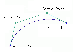
Bezier spline is a way to define a curve by sequence of
two end points and one or more control points which control
the curve.
Two end points are called Anchor Points.
The bezier splines with two control points are called Cubic Bezier Spline.
Note: this approach is entirely synthetic!
Using the vector is reasonable, but what makes 3 a magic number?
While cute, this derivation was not very natural
Thus, every point on the curve is a linear combination of the control points.The weights of this combination are all positive.The sum of these weights is 1.Therefore, the curve is a convex combination of the control points! |
 |
Some of theses properties may sound somewhere obvious, but they are presented here because they are still valid for Bézier curves of higher degree
The degree of the polynomial is always one less than the number of control points. In computer graphics, we generally use degree 3. Quadratic curves are not flexible enough and going above degree 3 gives rises to complications and so the choice of cubics is the best compromise for most computer graphics applications.
Moving any control point affects all of the curve to a greater or lesser extent. All the basis functions are everywhere non-zero except at the point u = 0 and u = 1
This is the basis of the intuitive 'feel' of a Bézier curve interface.
The curve does not oscillate about any straight line more often than the control point polygon
The curve is transformed by applying any affine transformation (that is, any combination of linear transformations) to its control point representation. The curve is invariant (does not change shape) under such a transformation.
As soon as you move one control point, you affect the entire curve
To learn more..."Cubic Bezier Patches Used to Draw Utah Teapot"
Bi(u) = (u^3)/6Bi-1(u) = (-3*(u^3) + 3*(u^2) + 3*u +1)/6 Bi-2(u) = (3*(u^3) - 6*(u^2) +4)/6 Bi-3(u) = (1 - u)^3/6 |
 |
Bi(u) = (u^3)/6Bi-1(u) = (-3*((u-1)^3) + 3*((u-1)^2) + 3*(u-1) +1)/6 Bi-2(u) = (3*((u-2)^3) - 6*((u-2)^2) +4)/6 Bi-3(u) = (1 - (u-3))^3/6 |
 |
Bi(u) = (u^3)/6
Bi-1(u) = (-3*((u-1)^3) + 3*((u-1)^2) + 3*(u-1) +1)/6
Bi-2(u) = (3*((u-2)^3) - 6*((u-2)^2) +4)/6
Bi-3(u) = (1 - (u-3))^3/6

B(u) = Bi(u) when 0 <= u < 1,
       Bi-1(u) when 1 <= u < 2,
       Bi-2(u) when 2 <= u < 3,
       Bi-3(u) when 3 <= u < 4
|
 |
Bi(u) = (u^3)/6
Bi1(u) = (-3*((u-1)^3) + 3*((u-1)^2) + 3*(u-1) +1)/6
Bi2(u) = (3*((u-2)^3) - 6*((u-2)^2) +4)/6
Bi3(u) = (1 - (u-3))^3/6


B(u) = Bi(u) when 0 <= u < 1,
       Bi1(u) when 1 <= u < 2,
       Bi2(u) when 2 <= u < 3,
       Bi3(u) when 3 <= u < 4

B1(u) = B(u-1)
B2(u) = B(u-2)
B3(u) = B(u-3)
B4(u) = B(u-4)
|
 |
To calculate the curve at any parameter t we place a gaussian
curve over the parameter space. This curve is actually an approximation of a
gaussian; it does not extend to infinity at each end, just to +/- 2 by using
the following equations:
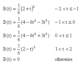
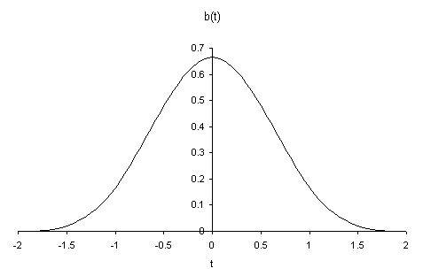
This curve peaks at a value of 2/3, and at +/- 1 its value is 1/6. When this
curve is placed over the array of control points, it gives the weighting of
each point. As the curve is drawn, each point will in turn become the heaviest
weighted, therefore we gain more local control.
Some of the properties that we listed for Bézier Curves apply to B-spline curves, in particular :
The curve follows follows the shape of the control point polygon and is constrained to lie in the convex hull of the control points.
The curve does not oscillate about any straight line more often than the control point polygon
The curve is transformed by applying any affine transformation (that is, any combination of linear transformations) to its control point representation.
In addition B-splines posses the following properties
A B-Spline curve exhibits local control - a control point is connected to four segments (in the case of a cubic) and moving a control point can influence only these segments
Bézier |
B-Spline |
(n - 1)/3 |
n-3 |
In CAGD applications, a curve may have a so complicated shape that it cannot be represented by a single Bézier cubic curve since the shape of a cubic curve is not rich enough. Increasing the degree of a Bézier curve adds flexibility to the curve for shape design. However, this will significantly increase processing effort for curve evaluation and manipulation. Furthermore, a Bézier curve of high degree may cause numerical noise in computation. For these reasons, we often split the curve such that each subdivided segment can be represented by a lower degree Bézier curve. This technique is known as piecewise representation. A curve that is made of several Bézier curves is called a composite Bézier curve or a Bézier spline curve. In some area (e.g., computer data exchange), a composite Bézier cubic curve is known as the PolyBézier. If a composite Bézier curve of degree n has m Bézier curves, then the composite Bézier curve has in total m×n+1 control vertices.
A curve with complex shape may be represented by a composite Bézier curve formed by joining a number of Bézier curves with some constraints at the joints. The default constraint is that the curves are jointed smoothly. This in turn requires the continuity of the first-order derivative at the joint, which is known as the first-order parametric continuity. We may relax the constraint to require only the continuity of the tangent directions at the joint, which is known as the first-order geometric continuity. Increasing the order of continuity usually improves the smoothness of a composite Bézier curve. Although a composite Bézier curve may be used to describe a complex shape in CAGD applications, there are primarily two disadvantages associated the use of the composite Bézier curve:
These disadvantages can be eliminated by working with spline curves. Originally, a spline curve was a draughtsman's aid. It was a thin elastic wooden or metal strip that was used to draw curves through certain fixed points (called nodes). The resulting curve minimizes the internal strain energy in the splines and hence is considered to be smooth. The mathematical equivalent is the cubic polynomial spline. However, conventional polynomial splines are not popular in CAD systems since they are not intuitive for iterative shape design. B-splines (sometimes, interpreted as basis splines) were investigated by a number of researchers in the 1940s. But B-splines did not gain popularity in industry until de Boor and Cox published their work in the early 1970s. Their recurrence formula to derive B-splines is still the most useful tool for computer implementation.
It is beyond the scope of this section to discuss different ways of deriving B-splines and their generic properties. Instead, we shall take you directly to the definition of a B-spline curve and then explain to you the mathematics of B-splines. Given M control vertices (or de Boor points) di (i = 0,1,Ľ,M-1), a B-spline curve of order k (or degree n = k-1) is defined as
|
|
As we said previously, there are several methods to derive the B-spline basis functions Ni,k(u) in terms of the knot vector. We present only the recursive formula derived by de Boor and Cox as follows:
|
|
|||||||