Radiosity OverView Part 2
Reference: SIGGRAPH 1993 Education Slide Set, by Stephen Spencer
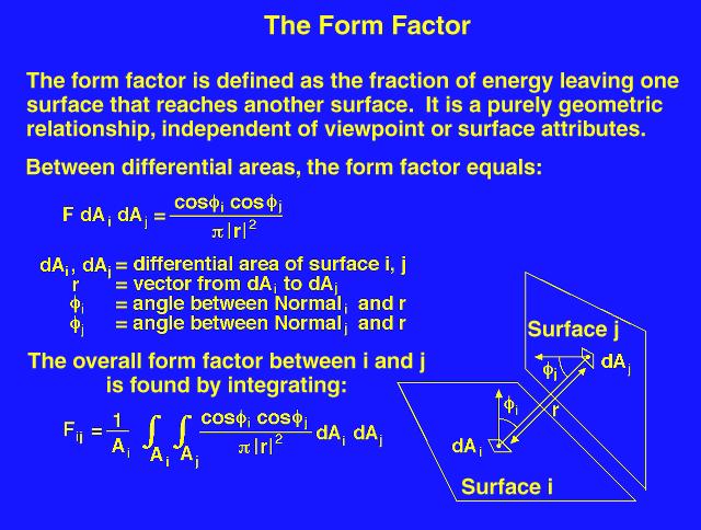
Slide 7 : The Form Factor.
The "form factor" describes the fraction of energy which leaves one surface and arrives at a second surface. It takes into account the distance between the surfaces, computed as the distance between the center of each of the surfaces, and their orientation in space relative to each other, computed as the angle between each surface's normal vector and a vector drawn from the center of one surface to the center of the other surface. It is a dimensionless quantity.
The form factor, as initially shown, describes the form factor between two differential areas; that is, a point-to-point form factor. To use this form factor with surfaces which have a positive area, the equation must be integrated over one or both surface areas. The form factor between a point on one surface and another surface with positive area can be used if the assumption is made that the single point is representative of all of the points on the surface.
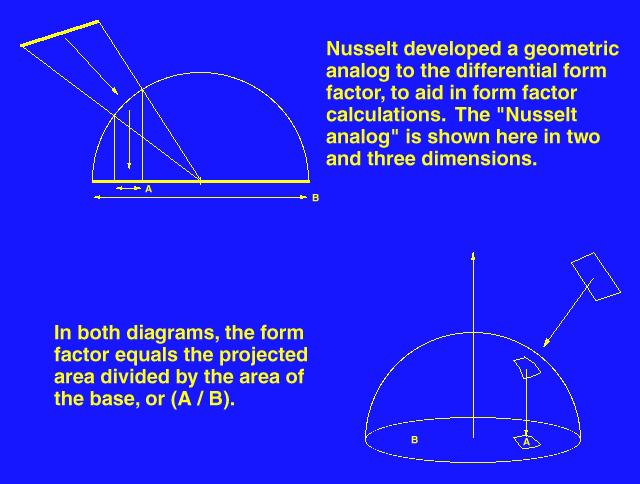
Slide 8 : The Nusselt Analog.
Differentiation of the basic form factor equation is difficult even for simple surfaces. Nusselt developed a geometric analog which allows the simple and accurate calculation of the form factor between a surface and a point on a second surface.
The "Nusselt analog" involves placing a hemispherical projection body, with unit radius, at a point on a surface. The second surface is spherically projected onto the projection body, then cylindrically projected onto the base of the hemisphere. The form factor is, then, the area projected on the base of the hemisphere divided by the area of the base of the hemisphere.
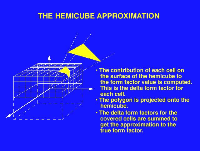
Slide 9 : The Hemicube.
The "hemicube" form factor calculation method involves placing the center of a cube at a point on a surface, and using the upper half of the cube (the "hemicube" which is visible above the surface) as a projection body as defined by the "Nusselt analog."
Each face of the hemicube is subdivided into a set of small, usually square ("discrete") areas, each of which has a pre-computed form factor value. When a surface is projected onto the hemicube, the sum of the form factor values of the discrete areas of the hemicube faces which are covered by the projection of the surface is the form factor between the point on the first surface (about which the cube is placed) and the second surface (the one which was projected).
The speed and accuracy of this method of form factor calculation can be affected by changing the size and number of discrete areas on the faces of the hemicube.
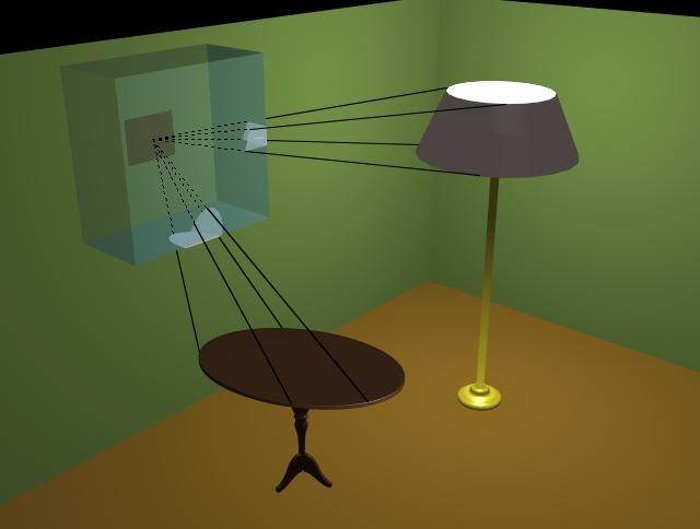
Slide 10 : The Hemicube In Action.
This illustration demonstrates the calculation of form factors between a particular surface on the wall of a room and several surfaces of objects in the room.
A standard radiosity image generation algorithm will compute the form factors from a point on a surface to all other surfaces, by projecting all other surfaces onto the hemicube and storing, at each discrete area, the identifying index of the surface that is closest to the point. When all surfaces have been projected onto the hemicube, the discrete areas contain the indices of the surfaces which are ultimately visible to the point. From there the form factors between the point and the surfaces are calculated.
For greater accuracy, a large surface would typically be broken into a set of small surfaces before any form factor calculation is performed.
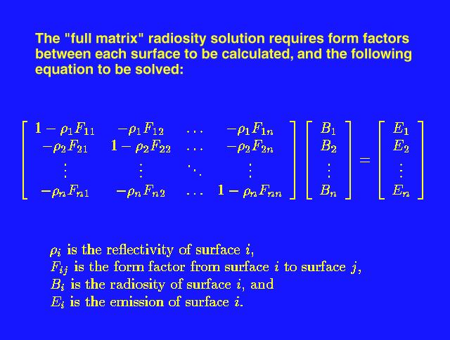
Slide 11 : The "Full Matrix" Radiosity Algorithm.
Two classes of radiosity algorithms have been developed which will calculate the energy equilibrium solution in an environment.
The "full matrix" radiosity solution calculates the form factors between each pair of surfaces in the environment, then forms a series of simultaneous linear equations, as shown in the upper figure. This matrix equation is solved for the "B" values, which can be used as the final intensity (or color) value of each surface.
This method produces a complete solution, at the substantial cost of first calculating form factors between each pair of surfaces and then the solution of the matrix equation. Each of these steps can be quite expensive if the number of surfaces is large: complex environments typically have upwards of ten thousand surfaces, and environments with one million surfaces are not uncommon. This leads to substantial costs not only in computation time but in storage.
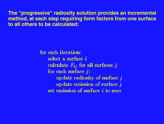
Slide 12 : The "Progressive" Radiosity Algorithm.
The "progressive" radiosity solution is an incremental method, yielding intermediate results at much lower computation and storage costs. Each iteration of the algorithm requires the calculation of form factors between a point on a single surface and all other surfaces, rather than all N-squared form factors (where "N" is the number of surfaces in the environment). After the form factor calculation, radiosity values for the surfaces of the environment are updated.
This method will eventually produce the same complete solution as the "full matrix" method, though, unlike the "full matrix" method, it will also produce intermediate results, each more accurate than the last. It can be halted when the desired approximation is reached. It also exacts no large (again, N-squared) storage cost.
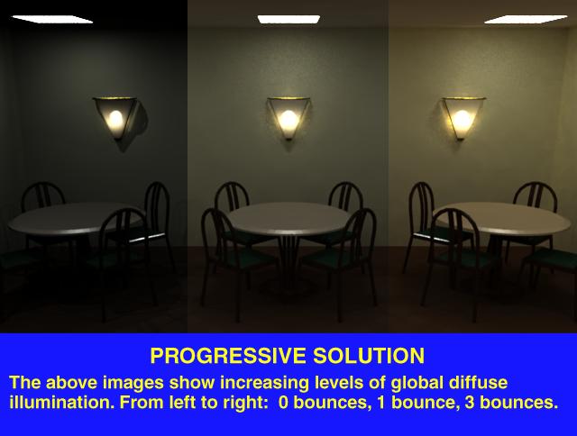
Slide 13 : Progressive Radiosity Examples.
This slide illustrates the iterative nature of the progressive method. The composite image shows that as the number of iterations increase, the accuracy of the intensity solution (and, hence, the resulting image) also increases. Of particular interest is the contribution of the color of the walls of the room to the overall color of the room in the right-most section of the composite image.
This image was created by calculating three separate but images, each halted at a different stage of rendering, and composited together afterwards.
[ OverView Part 1 ] [ OverView Part 2 UP ][ OverView Part 3 ]