Usual Graphics Pipeline and its Z buffer algo
Different classifications of globals illuminations model
Raytracing
Radiosity
Usual Graphics Pipeline and its Z buffer algoDifferent classifications of globals illuminations modelRaytracingRadiosity |
|
The painter's algorithm, sometimes called depth-sorting,
gets its name from the process which an artist renders a scene using oil paints.
First, the artist will paint the background colors of the sky and ground. Next,
the most distant objects are painted, then the nearer objects, and so forth.
Note that oil paints are basically opaque, thus each sequential layer completely
obscures the layer that its covers. A very similar technique can be used for
rendering objects in a three-dimensional scene. First, the list of surfaces
are sorted according to their distance from the viewpoint. The objects are
then painted from back-to-front.
While this algorithm seems simple there are many subtleties. The first issue
is which depth-value do you sort by? In general a primitive is not entirely
at a single depth. Therefore, we must choose some point on the primitive to
sort by.
1. Sort by the minimum depth extent of the polygon
2. Sort by the maximum depth extent of the polygon
3. Sort by the polygon's centriod (Sum(vi, i = 1..N)/N)
But the main issue is that it easy to face some absurdity like Triangle1 cover
part of Triangle2 which cover part of Triangle3 wich cover part of triangle1
The basic idea is to test the z - depth of each surface to determine the closest (visible) surface. Declare an array z buffer(x, y) with one entry for each pixel position. Initialize the array to the maximum depth. Note: if have performed a perspective depth transformation then all z values 0.0 <= z (x, y) <="1.0". So initialize all values to 1.0. Then the algorithm is as follows:
for each polygon P
  for each pixel (x, y) in P
    compute z_depth at x, y
    if z_depth < z_buffer (x, y) then
       set_pixel (x, y, color)
       z_buffer (x, y) <= z_depth
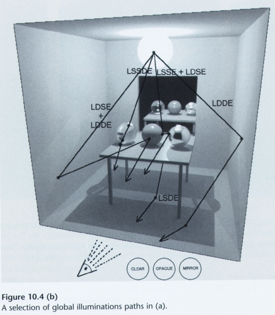 |
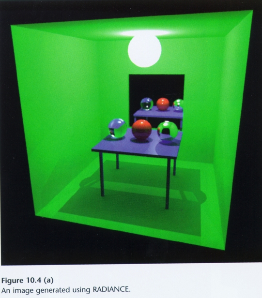
How do we accurately simulate all light interactions between objects?
Which are handled by ray tracing? Which by radiosity? |
First, let’s introduce some notation for paths. Each
path is terminated by the eye
and a light.
E - the eye.
L - the light.
Each bounce involves an interaction with a surface. We characterize the interaction
as either reflection or transmission. There are different types of reflection
and
transmission functions. At a high-level, we characterize them as
D - diffuse reflection or transmission
G - glossy reflection or transmission
S - specular reflection or refraction
Diffuse implies that light is equally likely to be scattered in any direction.
Specular
implies that there is a single direction; that is, given an incoming direction
there is
a unique outgoing direction. Finally, glossy is somewhere in between.
Particular ray-tracing techniques may be characterized by the paths that they
consider.
Appel Ray casting: E(D | G)L
Whitted Recursive ray tracing: E[S*](D | G)L
Kajiya Path Tracing: E[(D | G | S) + (D | G)]L
Goral Radiosity: ED*L
The set of traced paths are specified using regular expressions, as was first
proposed
by Shirley. Since all paths must involve a light L, the eye E, and at least
one
surface, all paths have length at least equal to 3.
A nice thing about this notation is that it is clear when certain types of paths
are not traced, and hence when certain types of light transport is not considered
by the algorithm. For example, Appel’s algorithm only traces paths of length
3,
ignoring longer paths; thus, only direct lighting is considered. Whitted’s
algorithm
traces paths of any length, but all paths begin with a sequence of 0 or more
mirror
reflection and refraction steps. Thus, Whitted’s technique ignores paths
such as
the following EDSDSL or E(D | G)* L. Distributed ray tracing and path tracing
includes multiple bounces involving non-specular scattering such as E(D | G)*
L.
However, even these methods ignore paths of the form E(D | G)S* L; that is,
multi-ple
specular bounces from the light source as in a caustic. Obviously, any technique
that ignores whole classes of paths will not correctly compute the solution
to the
rendering equation.
First Pass - formalized by Rushmeier and Torrance
Diffuse Transmission
Specular Transmission
Specular Reflection
With these extensions, we can now account for:
Once this pass is complete, we then perform the 2nd pass to compute specular - specular and diffuse - specular
Specular - specular is given by ray tracing
For diffuse - specular, we would need to send out many rays from the point through the hemisphere around the point, weight the rays by the bidirectional specular reflectivity, then sum them together.
![]()
we can rewrite this equation
as
![]() where R
is the linear integral operator
where R
is the linear integral operator
rearranging terms gives: 
.
Local Reflection Models
.
only first 2 terms are used
X is the eyepoint
![]()
the g(epsilon) term is non-zero only for light sources
R1 operates on (epsilon) rather than g, so shadows are not computed
Basic Ray Tracing
![]()
Radiosity
The Extended Two-Pass Algorithm (Sillion 1989)
.
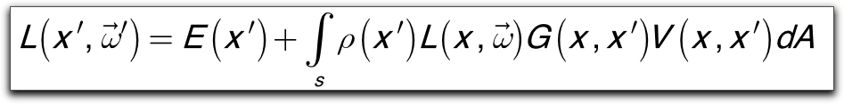
The general equation used is:
![]()
p(x, x', x'') = pd(x') + ps(x, x', x'')

bidirectional   diffuse    specular
reflectivity
  function
In the first pass, extended form factors are used to compute diffuse to diffuse interaction that has any number of specular transfers inbetween
extended form factors: Diffuse - specular* - diffuse
The 2nd pass uses standard ray tracing to compute specular transfer
 |
The entire beam can simply reflect. |
 |
A portion of the out-going beam can be blocked. |
 |
A portion of the incoming beam can be blocked.
|
 The electric
field of light has a magnetic field associated with it (hence the name electromagnetic).
The electric
field of light has a magnetic field associated with it (hence the name electromagnetic).
Hyperphysics : http://hyperphysics.phy-astr.gsu.edu/hbase/vision/photomcon.html
 |
 |
|
|
 |
|
 |
Ray TracingEffects needed for Realism
|
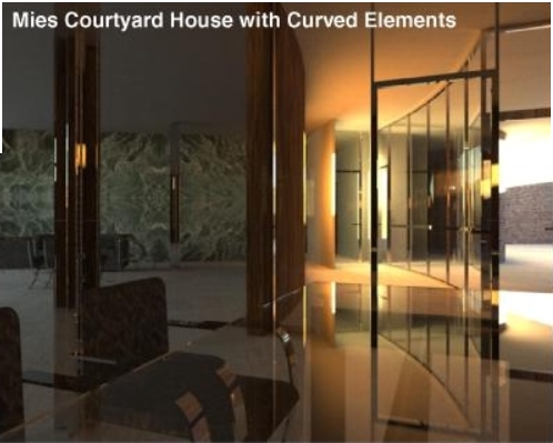 |
| The light of Mies van der Rohe / Modeling: Stephen Duck / Rendering: Henrik Wann Jensen |
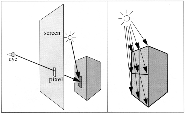
Ray Tracing is a global illumination based rendering method. It traces rays of light from the eye back through the image plane into the scene. Then the rays are tested against all objects in the scene to determine if they intersect any objects. If the ray misses all objects, then that pixel is shaded the background color. Ray tracing handles shadows, multiple specular reflections, and texture mapping in a very easy straight-forward manner.
Note that ray tracing, like scan-line graphics, is a point sampling algorithm. We sample a continuous image in world coordinates by shooting one or more rays through each pixel. Like all point sampling algorithms, this leads to the potential problem of aliasing, which is manifested in computer graphics by jagged edges or other nasty visual artifacts.
In ray tracing, a ray of light is traced in a backwards direction. That is, we start from the eye or camera and trace the ray through a pixel in the image plane into the scene and determine what it hits. The pixel is then set to the color values returned by the ray.
|
 |
Ray CastingCompared to Forward Mapping, there are other ways to compute views of scenes defined by geometric primitives. One of the most common is ray-casting. Ray-casting searches along lines of sight, or rays, to determine the primitive that is visible along it.Properties of ray-casting:
|
Usual Graphics Pipeline
Ray Casting
E (D | G) L |
In a ray-casting renderer the following process takes
place.
1. For each "Screen-space" pixel compute the equation of the "Viewing-space"
ray.
2. For each object in the display-list compute the intersection of the given
ray
3. Find the closest intersection if there is one
4. Illuminate the point of intersection
|
Appel 68 |
For each pixel
Recursive
|
E[S*](D | G)LTurner Whitted (1980)  Figure from Andrew S. Glassner, "An Overview of Ray Tracing" in An Introduction to Ray Tracing, Andrew Glassner, ed., Academic Press Limited, 1989. |
A primary ray is shot through each pixel and tested for intersection against all objects in the scene. If there is an intersection with an object then several other rays are generated. Shadow rays are sent towards all light sources to determine if any objects occlude the intersection spot. In the figure below, the shadow rays are labeled Si and are sent towards the two light sources LA and LB. If the surface is reflective then a reflected ray, Ri, is generated. If the surface is not opaque, then a transmitted ray, Ti, is generated. Each of the secondary rays is tested against all the objects in the scene.
The reflective and/or transmitted rays are continually generated until the ray leaves the scene without hitting any object or a preset recursion level has been reached. This then generates a ray tree, as shown below.
The appropriate local illumination model is applied at each level and the resultant intensity is passed up through the tree, until the primary ray is reached. Thus we can modify the local illumination model by (at each tree node)
I = Ilocal + Kr * R + Kt * T where R is the intensity of light from the reflected ray and T is the intensity of light from the transmitted ray. Kr and Kt are the reflection and transmission coefficients. For a very specular surface, such as plastic, we sometimes do not compute a local intensity, Ilocal, but only use the reflected/transmitted intensity values.
| Scene with no reflection rays |  |
Scene with one layer of reflection |  |
|---|---|---|---|
| Scene with two layers of reflection |  |
The first step is to create the model of the image. One should not hardcode objects into the program, but instead use an input file.
For each pixel we must generate a primary ray and test for intersection with all of the objects in the scene. If there is more than one ray-object intersection then we must choose the closest intersection (the smallest positive value of t).To ensure that there are no objects intersected in front of the image plane (this is called near plane clipping), we keep the distance of the primary ray to the screen and test all intersections against this distance. If the t value is less than this distance, then we ignore the object.
If there is an intersection then we must compute the shadow rays and the reflection rays.
The shadow ray is a ray from the point of intersection to the light source. Its purpose is to determine if the intersection point is in the shadow of a particular light. There should be one shadow ray for each light source. The origin of the shadow ray is the intersection point and the direction vector is the normalized vector between the intersection point and the position of the light source. Note that this is the same as the light vector (L) that is used to compute the local illumination.
Compute the Local Illumination at each point, carry it
back to the next level of the ray tree so that the intensity I = Ilocal + Kr
* R + Kt * T . Note that Kr can be taken as the same as Ks.
For each color (R, G, B) I is in the range 0.0 <= I <= 1.0. This must
be converted to an integer value of 0 <= I <= 255. The result is then
written to the output file.
The output file will consist of three intensity values (Red, Green, and Blue) for each pixel. For a system with a 24-bit framebuffer this file could be directly displayed. However, for a system with an 8-bit framebuffer, the 24-bit image must be converted to an 8 bit image, which can then be displayed. A suggested format for the output file is the Microsoft Windows 24-bit BMP image file format.
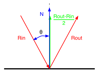
Rin an Rout are unit vector
You can form a losange with Rin and Rout

The source code for the applet can be found here.
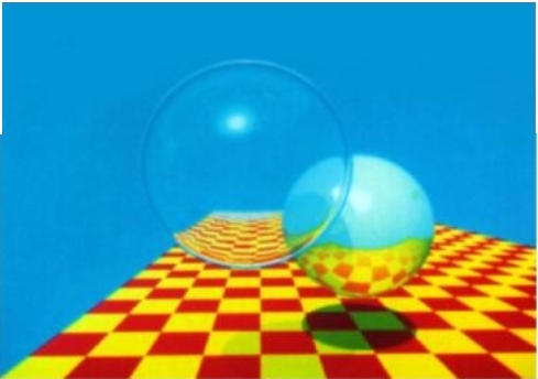
Advantages of Ray Tracing:
Spheres were one of the first bounding volumes used in raytracing, because of their simple ray-intersection and the fact that only one is required to enclose a volume. |
 |
 |
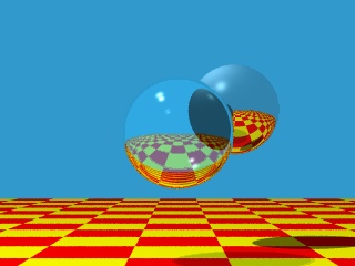
However, spheres do not usually give a very tight fitting bounding volume. More frequently, axis-aligned bounding boxes are used. Clearly, hierarchical or nested bounding volumes can be used for even greater advantage. |
References:
Cohen and Wallace, Radiosity and Realistic Image Synthesis
Sillion and Puech, Radiosity and Global Illumination
Thanks to Leonard McMillan for the slides
Thanks to François Sillion for images
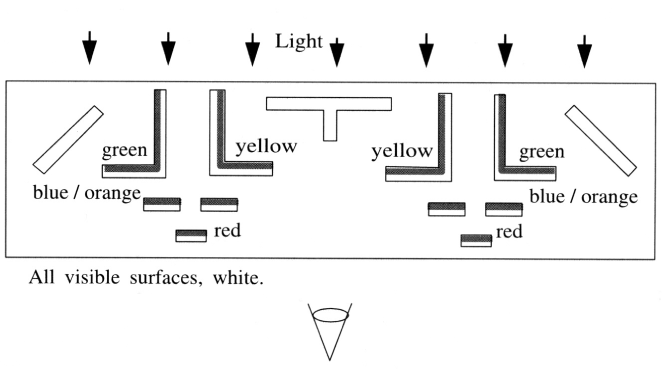
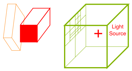
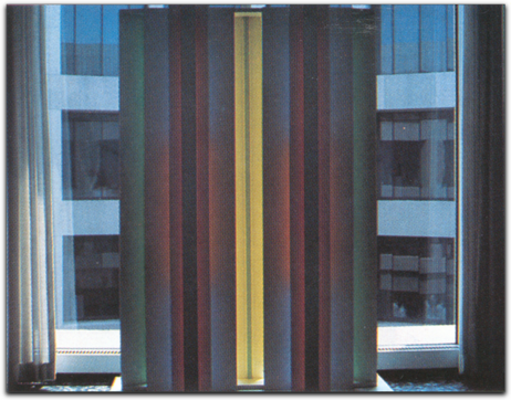
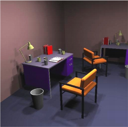
A powerful demonstration introduced by Goral et al. of the differences between radiosity and traditional ray tracing is provided by a sculpture by John Ferren. The sculpture consists of a series of vertical boards painted white on the faces visible to the viewer. The back faces of the boards are painted bright colors. The sculpture is illuminated by light entering a window behind the sculpture, so light reaching the viewer first reflects off the colored surfaces, then off the white surfaces before entering the eye. As a result, the colors from the back boards “bleed” onto the white surfaces.
Original sculpture lit by daylight from the rear.
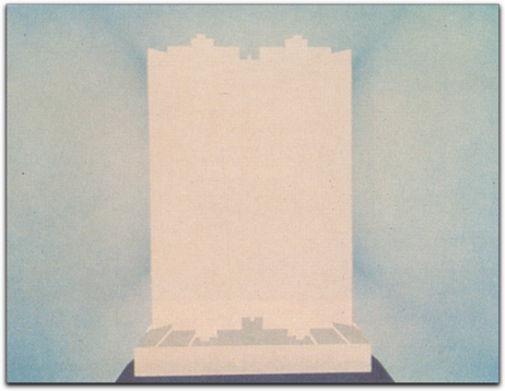
Ray traced image. A standard Ray tracer cannot simulate the interreflection of light between diffuse Surfaces.
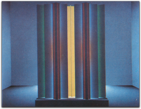
Image rendered with radiosity.
note color bleeding effects.
Because the solution is limited by the
view, ray tracing is often said to provide a view-dependent solution, although
this is somewhat misleading in that it implies that the radiance itself is
dependent on the view, which is not the case. The term view-independent refers
only to the use of the view to limit the set if locations and directions for
which the radiance is computed.
 |
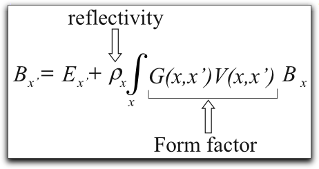
For an environment composed of diffuse surfaces, we have the basic radiosity relationship: |
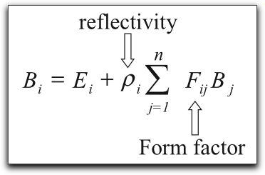
 |
For an environment that has been discretized into n patches, over which the radiosity is constant, (i.e. both B and E are constant across a patch), we have the basic radiosity relationship: |