eScience Lectures Notes : .
Managing Dynamic Shared State
Introduction
NVE
Shared State
Problem : Latency
Consistency-Throughput Tradeoff
High Consistency versus Highly Dynamic
Tradeoff Spectrum
3 Technics
Centralized Shared Repositories
Shared File Directory
Repository in Server Memory
Central server : Pull
Central server : Server Push the information
Virtual Repositories
Advantage and Drawback of Shared Repositories
Conclusion for Shared Repositories
Frequent State Regeneration / Blind Broadcasts
Explicit Object Ownership
Lock Manager
Update by Non-owner: Proxy Update
Update by Non-owner : Ownership Transfer
Reducing Broadcast Scope
Advantages of Blind Broadcasts
Disadvantages of Blind Broadcasts
Dead Reckoning
Dead Reckoning Issues
Prediction Techniques
Hybrid polynomial prediction
PHBDR (Position History-Based Dead Reckoning)
Limitations of Derivative Polynomials
Object-Specialized Prediction
The Phugoid model
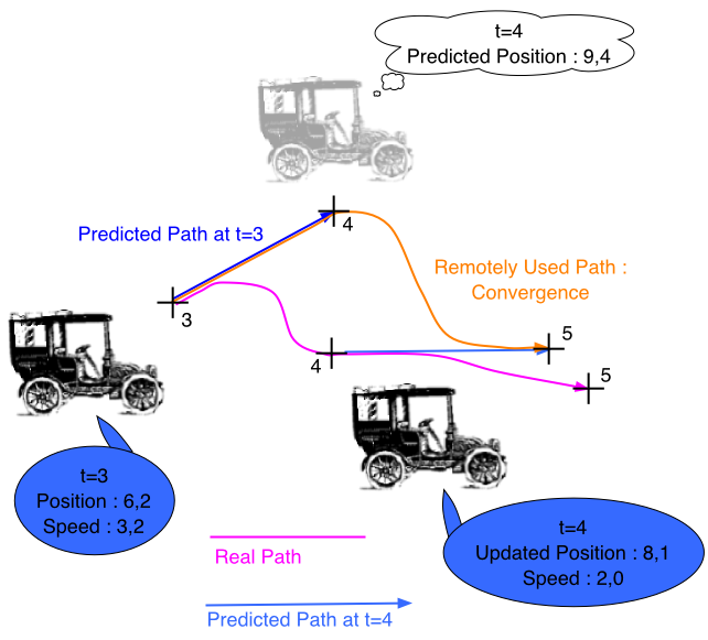
Convergence Algorithms
Linear convergence
Higher Level Convergence
Non-regular update packet transmission
Non-regular update packet transmission (2)
Dead Reckoning Conclusion
Conclusion
Managing Dynamic Shared State
Consistency-Throughput Tradeoff
3 different approaches
-
Centralized/Shared Repository
-
Frequent State Regeneration (Blind Broadcast)
-
Dead Reckoning
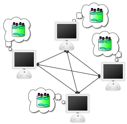
NVE
What are Networked Virtual Environment all about ?
-
Many participants scattered on different machines
-
All changing their own parameters (location, etc.)
-
All trying to see each other in real-time
Goal
-
Provide users with the illusion that they are all seeing the same things and interact with each other within that virtual space
Answer : Shared State
Shared State
The dynamic information that multiple hosts must maintain about the net-VE
Accurate dynamic shared state is fundamental to creating realistic virtual environments. It is what makes a VE “multi-user”.
Without Dynamic shared state, each user works independently and loses the illusion of being located in the same place and time as other users
Management is one of the most difficult challenges facing the net-VE designer. The trade off is between resources and realism.
How to make sure that the participating hosts keep a consistent view of the dynamic shared state
Example
-
Information of what and who is currently participating in the VE
-
Location and behaviour of Participant (object)
-
Shared environmental information- weather, terrain, etc.
Problem : Latency
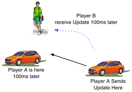
By the time the information arrives at the other player's machines, it is already obsolete.
Delay components in net-VE
|
Consistency-Throughput Tradeoff
 |
“It is impossible to allow dynamic shared state to change frequently and guarantee that all hosts simultaneously access identical versions of that state.”We can have either a dynamic world or a consistent world, but not both. |
"The more precisely the POSITION is determined,
the less precisely the MOMENTUM is known"
Werner Heisenberg : "Uncertainty Principle"
High Consistency versus Highly Dynamic
Player A moves and generates a location update.
To ensure consistency, player A must await acknowledgments.
If network lag is 100 ms, acknowledgment comes no earlier than 200 ms.
Therefore, player A can only update his state 5 times per second.
Far from the 30 Frame per second
For a highly dynamic shared state, hosts must transmit more frequent data updates.
To guarantee consistent views of the shared state, hosts must employ reliable data delivery.
NB. : Each host must either know the identity of all other participating hosts in the net-VE or a central server must be used as a clearing house for updates and acknowledgments.
Available network bandwidth must be split between these two constraints.
Tradeoff Spectrum
System characteristic |
Absolute consistency |
High update rate |
|---|---|---|
View consistency |
Identical at all hosts |
Determined by data received at each host |
Dynamic data support |
Low:limited by consistency protocol |
High:limited only by available bandwidth |
Network infrastructure requirements |
Low latency, high reliability, limited variability |
Heterogeneous network possible |
Number of participants supported |
Low |
Potentially high |
3 Technics
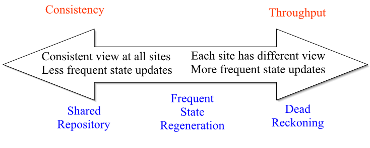
More Consistent More Dynamic
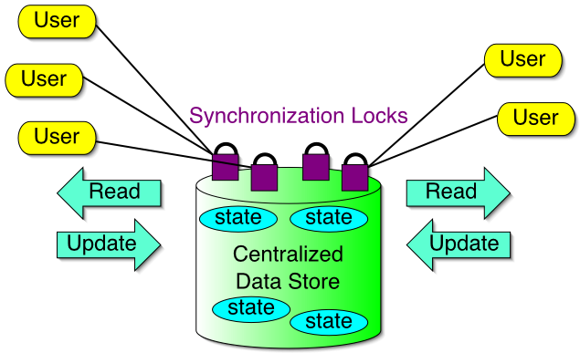
Centralized Shared Repositories
All hosts display identical views of the VE by making sure that all hosts see the same values for the shared state value at all times
Maintain shared state data in a centralized location.
Protect shared states via a lock manager to ensure ordered writes.
Three Techniques
|
 |
Shared File Directory : Hugh's Lab
File system : pull
A directory containing files that hold shared state
Absolute Consistency ! : Only one host can write data to the same file at a time.
Locate the file containing information and read/write the file data (file:user, object information)
Read and the reopen in write only mode
Maintain "lock" information for each file, and only one writer may hold that lock at a time
Ex. : NFS, AFS
Pros.
-
Simplest to program
-
Highest consistency
Cons.
-
Slow data update and access
-
Does not support many users
Constant need to open, update, close remote file
Repository in Server Memory
Instead of storing all of the VE's shared state in files, write a server process that simulates the behavior of a distributed file system
Each host maintains a TCP/IP connection to the server process and uses that connection to perform read and write operation on the shared state
Faster than Shared File because each host does not have to open and close each file remotely.
Don’t have to have locks. Server arbitrates.
Pros.
-
The server keep the current shared state in memory
-
The client no longer has to perform open and close operation on each file or unit of shared state
-
The server may support batched operation (multiple read and write in one request)
Cons.
-
If the server crashes, the current VE state will be lost
-
Maintaining a persistent TCP/IP connection to each client may strain server resources
Support small to medium-sized net VEsn
Central server : Client Pull Information
Clients pull information whenever they need it
Each client must make a request to the central state repository whenever it needs to access data.
Faster data update and access
The network VR project (NEC research lab.)
Use per-client FIFO queues to support "eventual consistency" state update delivery (incremental updates : position before speed)
Central server : Server Push the information
Each client maintain a local cache of the current net-VE state
The server "push" information to the clients over a reliable, ordered TCP/IP stream whenever the data is updated
Clients must request and obtain a lock before updating central state data
NB. Round Robin Passing Scheme : to ensure that all clients get an equal opportunity
to make shared state update
Immediate data access
Slower data update.
Shastra system (Purdue Univ.)
Virtual Repositories
Eliminate the centralized repository by placing it on a distributed consistency protocol by ensuring reliable message delivery, effective message dissemination, and global message ordering
AdvantagesEliminate the performance bottleneck introduced by accessing the single-host central repositoryEliminate the bandwidth bottleneck at the central repositoryPermit better fault tolerance |
 |
Advantage and Drawback of Shared Repositories
Advantage
-
Provide an easy programming model
-
Guarantee information absolute consistency
-
Does not impose any notion of data "ownership"
(Any host is able to update any piece of shared state by simply writing to the repository)
Drawback
-
Data access and update operations require an unpredictable amount of time to complete
-
Require considerable communication overhead due to reliable data delivery.
-
Vulnerable to single point failure
Conclusion for Shared Repositories
Most popular approach for maintaining shared state
Support a limited number of simultaneous users - on the order of 50 or 100
Each client's performance is closely linked to the performance of the other hosts
Approach is great for small-scale systems over LANs or engineering systems requiring highest levels of state consistency
Let's keep exploring the Local Cache idea, because, eventually...
Problem of the centralized repository
Too high overhead in communications and processor
Many applications don't require the "absolute consistency"
Example : Flight Simulator
In case of that error is limited and temporary
Frequent State Regeneration / Blind Broadcasts
Owner of each state transmits the current value asynchronously and unreliably at regular intervals.
Each host send its updated state frequently
No acknowledge packets are transmitted.
Clients cache the most recent update for each piece of the shared state.
Each host has its own cache to render the scene.
Hopefully, frequent state update compensate for lost packets.
No assumptions made on what information the other hosts have.
Asynchronous, unreliable blind broadcast is used
-
Usually the entire entity state is sent.
-
No acknowledgements
-
No assurances of delivery
-
No ordering of updates.
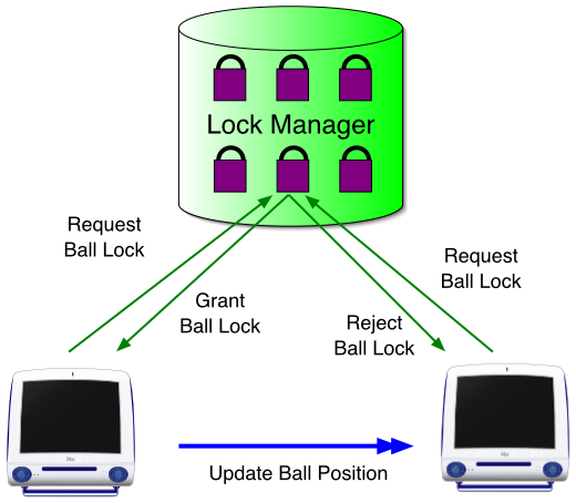
Explicit Object Ownership
With blind broadcasts, multiple hosts must not attempt to update an object at the same time.
Each host takes explicit ownership of one piece of the shared state (usually the user’s avatar).
To update an unowned piece of the shared state, either proxy updates or ownership transfer is employed.
Unless it owns the state, a host cannot update the state value
Lock Manager
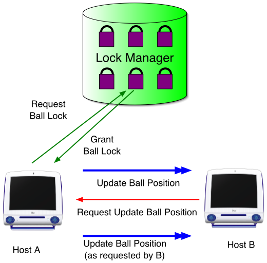
Update by Non-owner: Proxy Update
Use "private message" to entity ownerDecision by owner and broadcastingGood when Many host desire to update the state |
 |
Update by Non-owner : Ownership Transfer
Issue lock transfer request to lock managerExtra messaging overhead, compared with "proxy update"Good when Single host is going to make a series of updates
... Or the request of transfert could be done directly to the Lock Manager |
Reducing Broadcast Scope
Each host sends updates to all participants in the net-VE.
Reception of extraneous updates consumes bandwidth and CPU cycles.
Need to filter updates, perhaps at a central server (e.g. RING system) which forwards updates only to those who can “see” each other.
VEOS - epidemic approach- each host send info to specific neighbors.
Advantages of Blind Broadcasts
Simple to implement; requires no servers, consistency protocols or a lock manager (except for filter or shared items)
Can support a larger number of users at a higher frame rate and faster response time.
Systems using FSR
Real-time interaction among a small number of users
Extension of the single-user game
Dogfight, Doom, Diablo, etc.
Intra-vascular tele-surgery
Surgical catheter and an camera position
Video conferencing
Facial feature points of wire-frame model
Disadvantages of Blind Broadcasts
Requires large amount of bandwidth.
Network latency impedes timely reception of updates and leads to incorrect decisions by remote hosts.
Network jitter impedes steady reception of updates leading to ‘jerky’ visual behavior.
Assumes everyone broadcasting as the same rate which may be noticeable to users if it is not the case (this may be very noticeable between local users and distant destinations).
Dead Reckoning
State prediction techniques
Transmit state updates less frequently by using past updates to estimate (approximate) the true shared state.
Sacrificing accuracy of the shared state, but reducing message traffic.
Each host estimates entity locations based on past data.
No need for central server.
Dead Reckoning Issues
PredictionHow the object’s current state is computed based on previously received packets.ConvergenceHow the object’s estimated state is corrected when another update is received. |
 |
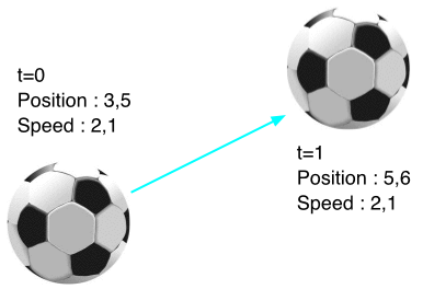
Prediction Techniques
Derivative Polynomial Approximation
Zero-order (position : simplest )
x(t + Dt) = x(t)
Frequent State Regeneration !
First-order (position+velocity)
x(t + Dt) = x(t) + Vx(t) * Dt
Second-order (position+velocity+acceleration)
x(t + Dt) = x(t) + Vx(t) * Dt + 1/2 * Ax(t) * (Dt)2
Most popular in NetVE
DIS Protocol
Higher Order Approximations
Jerk
Hybrid polynomial prediction
Choose between a first-order and a second-order prediction dynamically.
Need not be absolute
Instead of using a fixed prediction scheme, dynamically choose between first or second order based on object’s history.
Use first order when acceleration is negligible or acceleration information is unreliable (changes frequently).
PHBDR (Position History-Based Dead Reckoning)
Hybrid approach
Update packets only contain the object’s most recent position
Remote hosts estimate the instantaneous velocity and acceleration by averaging the position samples.
Reducing bandwidth
Improving prediction accuracy
(as “snapshot” velocities and accelerations can be misleading.)
Limitations of Derivative Polynomials
Why not use more terms?
greater bandwidth required
greater computational complexity
less accurate prediction since higher order terms are harder to estimate and errors have disparate impact
In many cases, More terms make things worse.
Example of second order polynomial equation : over time, the equation is more sensitive to the acceleration term than to the velocity term
Moreover, it is harder to get accurate instantaneous information about higher order derivatives (a user typicallt only controls an object's velocity and acceleration
The Jerk is all about human behavior
Do not take into account capabilities or limitations of objects.
Object-Specialized Prediction
Object behaviour may simplify prediction scheme (more information and constraint).
Choose different order for different type of object (ball, car, human ... )
Motion prediction does not require orientation information to be transmitted.
A plane’s orientation angle is determined solely by its forward velocity and acceleration.
Military flight manoeuvres simulation, The Phugoid model (Katz, Graham)
Land based objects need only two dimensions specified. (NPSNET)
Update packets only specify two dimensions to handle ground-based
tanks
The remote host adjust the object’s height and orientation to ensure that
object always travels smoothly along the ground
Drumstick position prediction(MIT)
Derivative polynomial approximation + ‘emergency’
message
Emergency message makes the computer disregard its current prediction whenever
a sudden change in the drum stick behaviour was detected
High-level state notification (acting)
Desired level of detail - often do not need to be precise with some aspects. Do we have to accurately model the flicker of the flames of a burning vehicle or is it enough to say it is on fire.
The same with smoke. Some VEs need to accurately model smoke, other do not.
Sometimes, remote host don’t need to model the precise
behaviour of the entity.
Dancing, firing, etc.
Remote hosts simply need to receive notification of the high-level state change.
These hosts are free to locally simulate the precise behaviour represented by
that state.
Dancing
Source of that document : http://www.math.sunysb.edu/~scott/Book331/Phugoid_model.html
The Phugoid model
The Phugoid model is a system of two nonlinear differential equations in a
frame of reference relative to the plane. Let v(t) be the speed
the plane is moving forward at time t, and ![]() (t) be the angle the nose makes with the horizontal. As
is common, we will suppress the functional notation and just write v
when we mean v(t), but it is important to remember that v
and
(t) be the angle the nose makes with the horizontal. As
is common, we will suppress the functional notation and just write v
when we mean v(t), but it is important to remember that v
and ![]() are functions of time.
are functions of time.
If we apply Newton's second law of motion (force = mass × acceleration) and examine the major forces acting on the plane, we see easily the force acting in the forward direction of the plane is
This matches with our intuition: When ![]() is negative, the nose is pointing down and the plane will accelerate
due to gravity. When
is negative, the nose is pointing down and the plane will accelerate
due to gravity. When ![]() > 0, the plane must fight against gravity.
> 0, the plane must fight against gravity.
In the normal direction, we have centripetal force, which is often expressed
as mv2/r, where r is the instantaneous radius
of curvature. After noticing that that
![]() = v/r, this can be expressed as
v
= v/r, this can be expressed as
v![]() , giving
, giving
Experiments show that both drag and lift are proportional to v2, and we can choose our units to absorb most of the constants. Thus, the equations simplify to the system

It is also common to use the notation ![]() for
for
![]() and
and
![]() for
for
![]() . We will use these notations interchangeably.
. We will use these notations interchangeably.
Translated from LaTeX by Scott Sutherland
2002-08-29
Convergence Algorithms
Tells us what to do to correct an inexact prediction:Trade-off between computational complexity and perceived smoothness of displayed entitiesZero-order(Snap) convergenceJumping from currently displayed location to its new location.Advantage: SimpleDisadvantage: Poorly models real world.
|
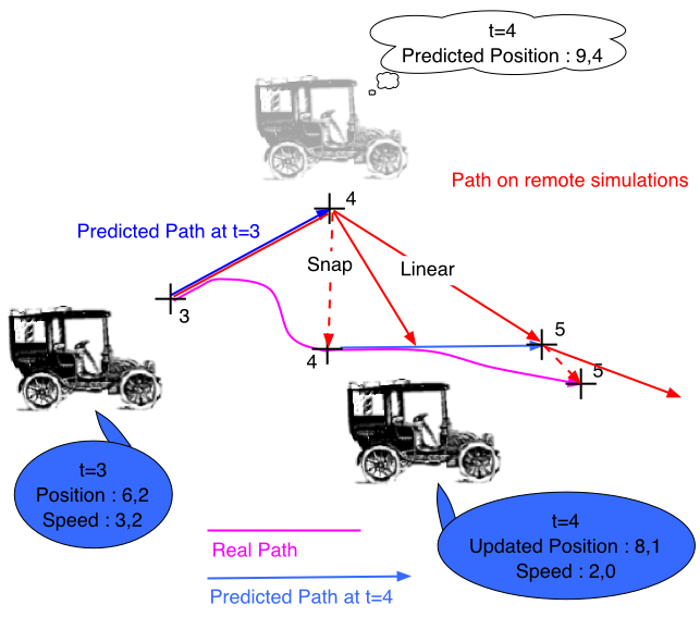 |
Linear convergence
Using future convergence point along the new predicted path.Advantage: Avoids jumpingDisadvantage: Does not prevent “sudden” or unrealistic changes in speed or direction.
|
|
Higher Level Convergence
Quadratic Curve fittingTo get more smooth convergence pathIssue : you still can not get C0 and C1 at both the two extremsCubic SplineAdvantage: Smoothest looking convergenceDisadvantage: Computationally expensiveNBChoice of convergence algorithm may vary within a VE depending on the entity type and characteristics. |
|
Non-regular update packet transmission
The source host can model the prediction algorithm being used by the remote host.
The host only needs to transmit updates when there is a significant divergence between the object’s actual position and the remote host’s predicted position.
Only transmit an update when an error threshold is reached or after a timeout period (heartbeat).
Entities must have a “heartbeat” otherwise cannot distinguish between live entities and ones that have left the system.
U.S. Army’s SIMNET, the DIS standard, NPSNET, PARADISE.
Non-regular update packet transmission (2)
Advantages
-
Reduction of update rates.
-
Guarantee about the overall accuracy of the remote state information.
-
Adaptation of the consistency-throughput based on the changing consistency demands of the net-VE
Problems
-
No update to be transmitted (the prediction algorithm is really good or the entity is not moving)
-
New participants will never receive any initial state.
-
Recipients cannot tell the difference between the network failure, no movement of entity, no change of object behavior.
To solve the problem, use the timeout on packet transmission ("heartbeat").
Dead Reckoning Conclusion
Reduction of bandwidth
Updates are sent less frequently.
Potentially larger number of players.
Each host does independent calculations
Limitation
No guarantee that all host share identical state about each entity – hosts can tolerate and adapt the potential discrepancy
More complex to develop, maintain, and evaluate.
Dead reckoning algorithm must often be customized based on the the behavior of the objects being modeled.
Collision detection difficult to implement.
Must have convergence to cover prediction errors.
Poor convergence methods lead to jerky movements and distract from immersion.
Conclusion
Shared state maintenance is governed by the Consistency-Throughput Tradeoff.
Three broad types of maintenance:
-
Centralized/Shared repository
-
Frequent State Regeneration(Blind Broadcast)
-
Dead Reckoning
The correct choice relies on balancing many issues including bandwidth, latency, data consistency, reproducibility, and computational complexity.